The change between week 3 and 4 was nothing too drastic, but had some key differences.

First, a PI controller was implemented. This only changed the code by simultaneously allowing the controller driver to take in speed and position, and then using a Ki value, could find the new duty cycle.

The more interesting change that was implemented during Week 4 was the use of a reference csv file that contained expected speed and position values at discrete points in time. This allowed us to try speed and positon tracking with our PI controller. in PC_FrontEnd.py, the data from the csv file was opened and resampled with a lower resolution. Since we aren't running the controller task at a 1ms interval, there was no need to use the fine resolution from the csv file. This also helped reduce the file size that was later loaded onto the Nucleo board. Once the file was on the Nucleo, the ctrlTask.py file would initialize by loading in all the data as 'reference values.' Each time the controller driver was called to find a new duty cycle, it would compare the current motor speeds and position against the reference data, and choose a new L value (duty cycle) accordingly. In order to find a reasonable reference time (since the file has a lower resolution), an interpolation method was created in order to find an appropriate reference speed and position for the current time value. This method is contained within the ctrlTask.py file.

Similar to Week3, the following files were implemented in order to properly control the motors and encoders.

–PC_FrontEnd.py

–main.py

–uiTask.py

–ctrlTask.py

–encoder.encoder

–controllerdriver.controllerdriver

–motor.motorDriver

–shares.py

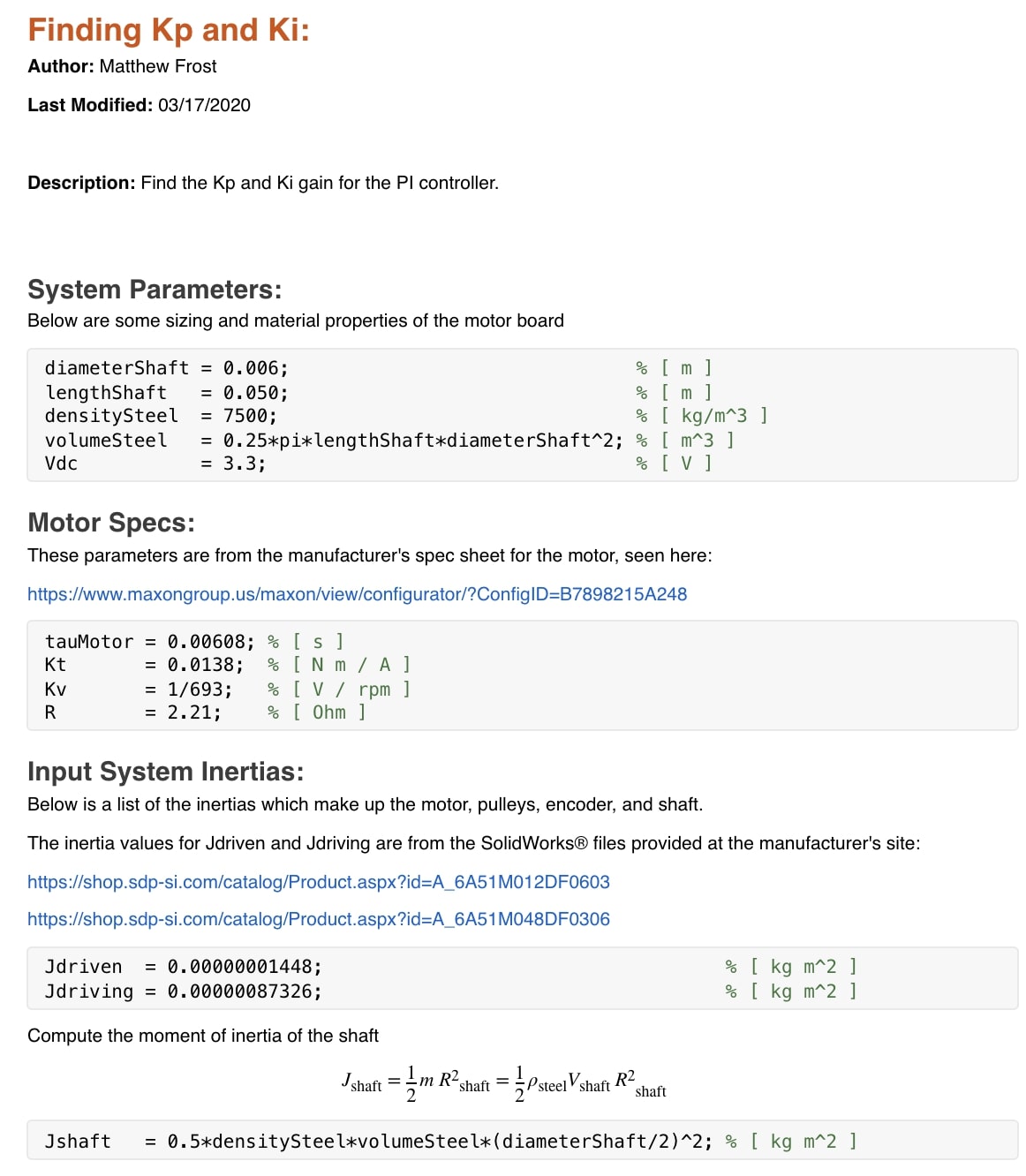
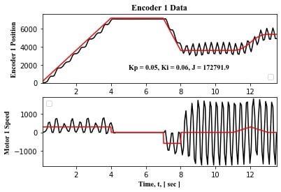
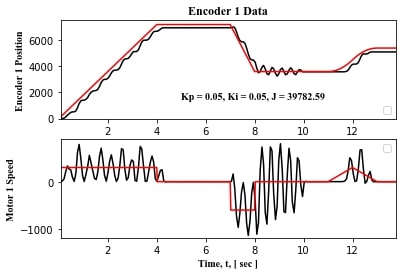
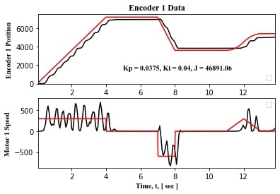
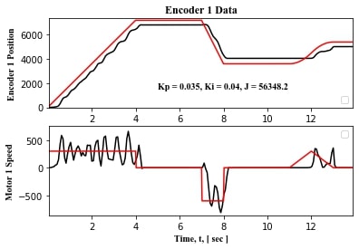
After the implementation of the classes and new controller setup was done, a few hours of iterating Kp and Ki was needed in order to attempt in finding a combination that allowed for the motor to accurately track the given profile. However, similar to week 3, the resolution of the data collection arose to be the leading cause in innaccurate tracking. Adjusting Ki and Kp definitely helped with reducing the error in the system, but if there was a way to get a finer resolution (say 5ms, instead of 20ms), the controller would correct and properly adjust the motor's trajectory to find the next duty cycle faster. Unfortunately, due to memory allocation failures on the Nucleo board, 20ms was the fastest period that could be run. Below are a few figures that show the tuning of the system, with the red line shown as the given profile. Kp and Ki were derived in a MATLAB script, as shown in the figure below, but due to assumptions about the friction in the system and unknown inertias, the values weren't much of a help.

Figure 1. Matlab Script to Derive Kp and Ki.

Additionally, and as can be seen on the plots, there is a J metric, which is meant to display the error in the system. This was described in the lab manual as the sum of the squares of the differences in expected and experienced speed/position. Because the units of speed and position aren't the same, and have completel difference magnitudes, the J metric is more weighted toward the error in the speed values, which is the reason that it's so high, while the position tracking worked fairly well.

Figure 2. Speed and Position Response with Kp = 0.05 and Ki = 0.06

Figure 3. Speed and Position Response with Kp = 0.05 and Ki = 0.05

Figure 4. Speed and Position Response with Kp = 0.0375 and Ki = 0.04

Figure 5. Speed and Position Response with Kp = 0.035 and Ki = 0.04

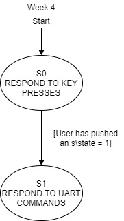
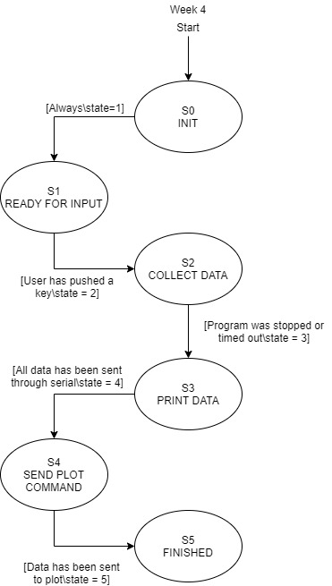
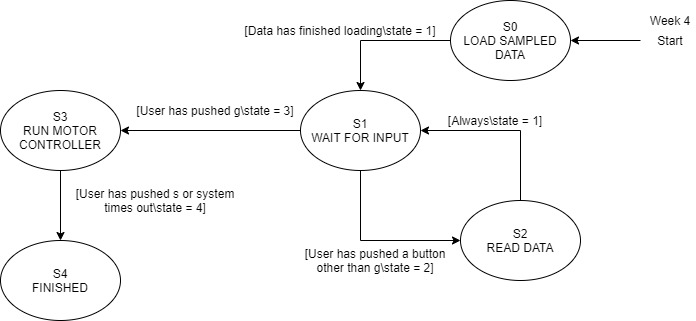
Below is a summary of the state diagrams utilized for the week. These stayed fairly consistent between weeks (the overall flow stayed the same, we were just exporting/sending more data with each week).

Figure 8. Week 4 Deliverable: Front End State Diagram

Figure 9. Week 4 Deliverable: UI Task State Diagram

Figure 10. Week 4 Deliverable: Controller Task State Diagram