Uncoupling and Linearizing EOMs

For the Jupyter Notebook file used to develop the content of this section, click here: Jupyter Notebook

In order to derive the closed-loop control, as well as simulate the expected response of the system, the system of equations derived in System Modeling: Kinetics and Kinematics must be decoupled and linearized in order to provide a representation of the sytem. To start, the system was put into space-state form with a vector x defined as holding the terms x (ball position), theta (platform rotation), and their first derivatives.

Also needed for linearization was an equilibrium point, which should be a stable 'resting' point of the system. In our case, the equilibrium point was the point where the ball is above the center of gravity of the platform with no velocity. Additionally, the angle and angular velocity of the platform are zero. This eases the Jacobian linearization process immensely, as the zeroth term of the Taylor series expansion is zero. Assuming that the ball doesn't deviate far from the equilibrium point, it can also be assumed that the higher order terms ("H.O.T.s") are negligible. This results in a Jacobian linearization process that can be followed in order to simulate and model the set of equations to describe the motion of the platform and ball. This consisted of getting an A and B matrix to represent the state of the system in the form of xdot = Ax + Bu, where u is the input vector, or motor torque.

Simulating the Motion of the System

Once the system has been put into the form of xdot = Ax + Bu, the system can be solved with an ordinary differential solver or linear time invariant system solver. This was performed in Jupyter with the 'lti' and 'lsim' functions within Python's sympy, numpy, and scipy.signal modules. These were solved for two initial cases:

The ball starts above the center of gravity with no velocity, and no tilt or angular velocity of the platform. There is no input torque from the motor.
The ball starts 5cm from the center of gravity with no velocity. The platform has no tilt angle or initial velocity. Additionally, there is no input torque from the motor.

As expected, the first case does not move the platform or ball, as it is already at the equilibrium condition. However, for the second case, the platform/ball system is not at equilibrium, and thus the position and velocity vectors are expected to be non-zero. This system was subsequently tested in an open- and closed-looped control system.

Open Loop Response

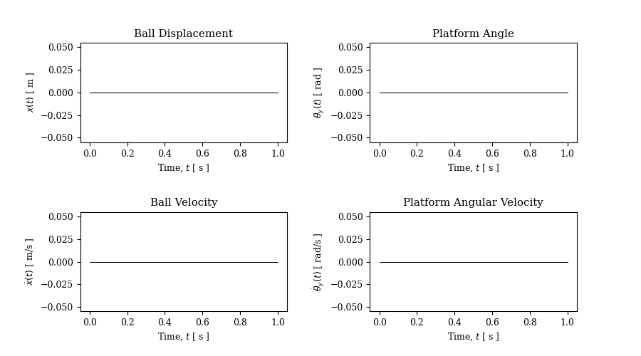
For the first test of the open loop system, the ball is modeled as starting in the center of the platfrom (or in other words, the center of mass of the ball is aligned with that of the platform). In this scenario, no feedback is needed as the ball is in the steady state position. See Figure 4 below for plots of all four state variables.

Figure 4. Open-loop response for steady-state position.

However, if the ball starts in any other position, the system cannot return to equilibrium, as there is no feedback to impose an opposite force to level the platform. Figure 5 below shows the system response for initial conditions in which the ball is offset horizontally from the center of the platform by 5 cm.

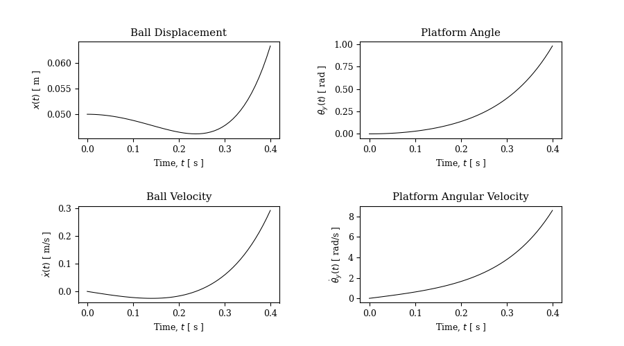
Figure 5. Open-loop response for non-zero initial conditions.

As is expected for this set of initial conditions and the open-loop configuration, we can see that the system is unstable.

Closed Loop Response

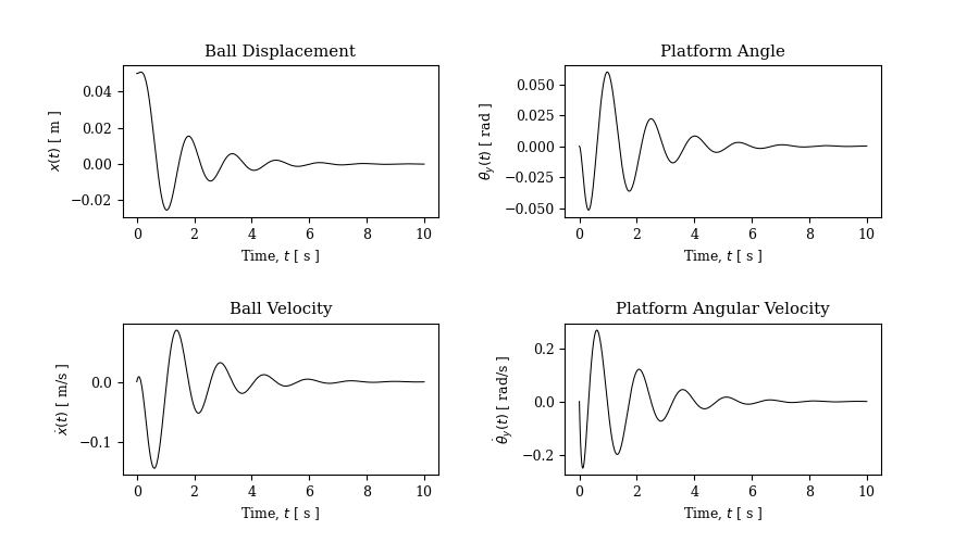
When ran in the closed-loop configuration, the system can now use the feedback of the velocity and position to return to equilibrium. For now, the closed-loop feedback was given as a function of the state variables, but in the future will be tuned to optimize the response of the system. Figure 6 displays the response of the system in the closed-loop control system. This system behaves as expected, as the response is a second-order response has a lot of overshoot as the platform jerks back and forth trying to stabilize the ball. Eventually, the controller is able to stabilize the system however, meaning the ball has returned back to equilibrium.

Figure 6. Closed-loop response for same non-zero initial conditions.

Continue to the next section here: Full-State Feedback